The Annotated Transformer Revisited

In this article we have an illustrated annotated look at the Transformer published in “Attention is all you need” in 2017 by Vaswani, Shazeer, Parmer, et al. The Transformer architecture was groundbraking as it achieves 28.4 BLEU on the WMT 2014 English-to-German translation task with comparatively very little training.

Even though it is eclipsed by the “Reformer: The Efficient Transformer” published by Nikita Kitaev, Łukasz Kaiser and Anselm Levskayain in this year/2020, it is still interesting to have a look at the fundamental idea of the comparatively “simple network architecture […] based solely on attention mechanisms”.

Overview

We will cover the setup and execute the Transformer implementation outlined in the given paper. We start with the excellent breakdowns created by Sasha Rush - The Annotated Transformer.

In contrast to the paper using Tensorflow (which also published its implementation 😊), we follow Sasha’s torch implementation as my impression is that more and more researchers are moving towards PyTorch. Everything will be contained in this annotated ipynb on Google Colab.

Breakdown

The simplified high-level overview of the transformer looks like this

with the layered setup of the Encoder and Decoder being as follows:

where the Fast Forward is a regular fully-connected neural network and the Self-Attention layer is searching for connections in the input while encoding. The decoder is identical except there being an additional Encoder-Decoder Attention between the prior two. This Encoder-Decoder Attention is the surrogate for attention decoder RNNs of previous architectures.

These can be stacked on top of each other. In the original paper 6 of each were stacked on top of each other. All with unique weights.

Now, we’ll create these using PyTorch. First we start with the bird’s-eye view:

class Encoder(nn.Module):
    "Core encoder is a stack of N layers"
    def __init__(self, layer, N):
        super(Encoder, self).__init__()
        self.layers = clones(layer, N)
        self.norm = LayerNorm(layer.size)

    def forward(self, x, mask):
        "Pass the input (and mask) through each layer in turn."
        for layer in self.layers:
            x = layer(x, mask)
        return self.norm(x)

class Decoder(nn.Module):
    "Generic N layer decoder with masking."
    def __init__(self, layer, N):
        super(Decoder, self).__init__()
        self.layers = clones(layer, N)
        self.norm = LayerNorm(layer.size)

    def forward(self, x, memory, src_mask, tgt_mask):
        for layer in self.layers:
            x = layer(x, memory, src_mask, tgt_mask)
        return self.norm(x)

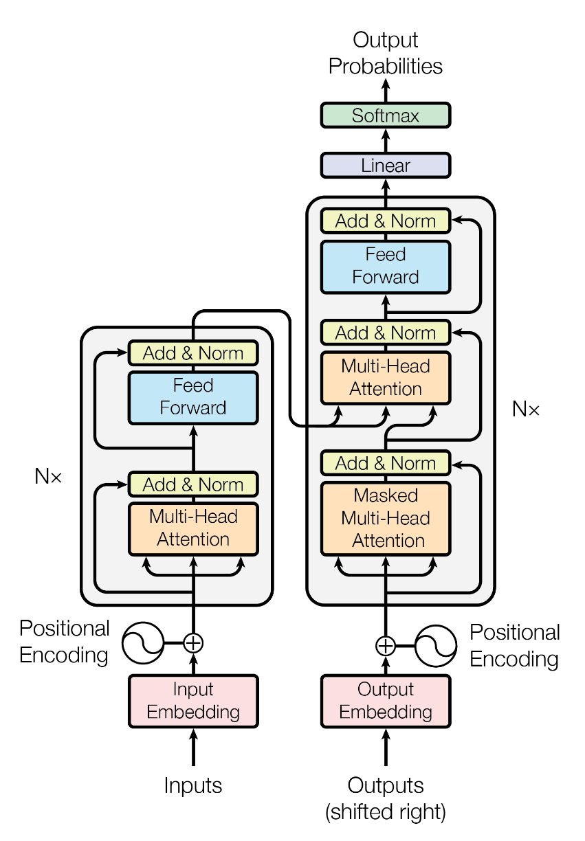
Above you can see two functions calls, which probably do not make sense immediately. That is clones(), which produces copies of layers, so we can stack them, and LayerNorm(), which corresponds to the yellow box of the original’s paper Fig 1.:

Fig 1: Architecture (src: Attention is all we need)

This Layer Normalization is similar to Batch Normalization and improves speed, perf and stability by applying a transformation which maintains the mean activation close to 0 and the activation standard deviation close to 1 followed by applying a slight bias based on the input.

The implementation of these two functions looks like this:

def clones(module, N):
    "Produce N identical layers."
    return nn.ModuleList([copy.deepcopy(module) for _ in range(N)])

class LayerNorm(nn.Module):
    "Construct a layernorm module (See citation for details)."
    def __init__(self, features, eps=1e-6):
        super(LayerNorm, self).__init__()
        self.a_2 = nn.Parameter(torch.ones(features))
        self.b_2 = nn.Parameter(torch.zeros(features))
        self.eps = eps

    def forward(self, x):
        mean = x.mean(-1, keepdim=True)
        std = x.std(-1, keepdim=True)
        return self.a_2 * (x - mean) / (std + self.eps) + self.b_2

As we introduced the original paper’s figure now, we can easily create the connection between our simplified model above and this structure. It’s interesting to note, that the final Encoder output is fed into each of the Encoder-Decoder Attention layers, which is called Multi-Head Attention in the original paper.

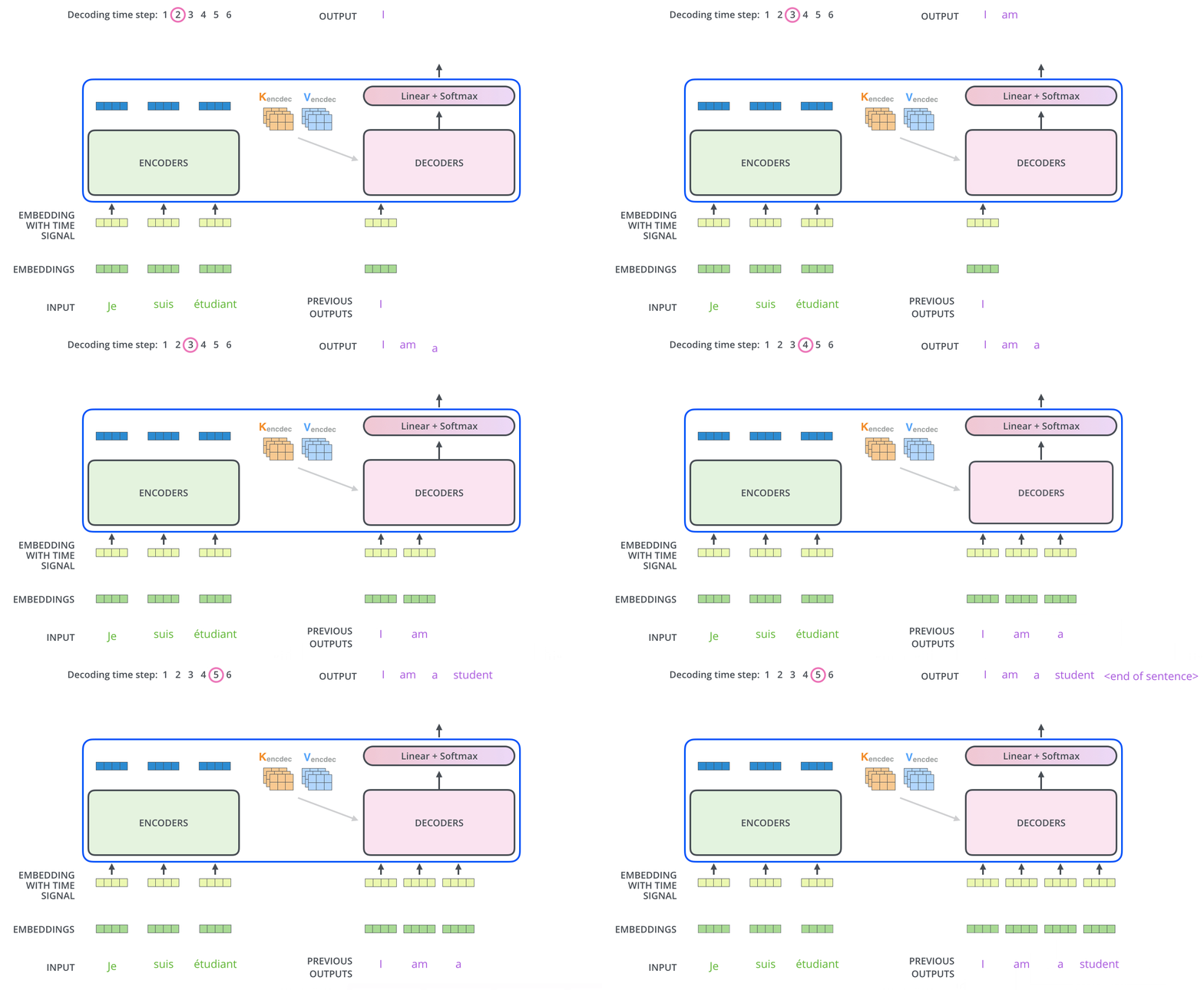
We’ll approach the original’s figure a bit more now. Of interest is, how the output is re-fed in to the decoders. Jay Alammar’s animation in his breakdown ‘The Illustrated Transformer’ is of great help to understand this concept:

Fig 2: Output embedding (src: Jay Alammar)

This also visualizes the RNN root of the concept.

But let’s get back to the implementation of the layers of the Encoder and Decoder. We start with the layers in the encoder:

class EncoderLayer(nn.Module):
    "Encoder is made up of self-attn and feed forward (defined below)"
    def __init__(self, size, self_attn, feed_forward, dropout):
        super(EncoderLayer, self).__init__()
        self.self_attn = self_attn
        self.feed_forward = feed_forward
        self.sublayer = clones(SublayerConnection(size, dropout), 2)
        self.size = size

    def forward(self, x, mask):
        "Follow Figure 1 (left) for connections."
        x = self.sublayer[0](x, lambda x: self.self_attn(x, x, x, mask))
        return self.sublayer[1](x, self.feed_forward)

Here one new function is introduced: SublayerConnection(), connecting all attention or feed-forward layers in each encoder or decoder layer.

The decoder layers look like this:

class DecoderLayer(nn.Module):
    "Decoder is made of self-attn, src-attn, and feed forward (defined below)"
    def __init__(self, size, self_attn, src_attn, feed_forward, dropout):
        super(DecoderLayer, self).__init__()
        self.size = size
        self.self_attn = self_attn
        self.src_attn = src_attn
        self.feed_forward = feed_forward
        self.sublayer = clones(SublayerConnection(size, dropout), 3)

    def forward(self, x, memory, src_mask, tgt_mask):
        "Follow Figure 1 (right) for connections."
        m = memory
        x = self.sublayer[0](x, lambda x: self.self_attn(x, x, x, tgt_mask))
        x = self.sublayer[1](x, lambda x: self.src_attn(x, m, m, src_mask))
        return self.sublayer[2](x, self.feed_forward)

Conclusion

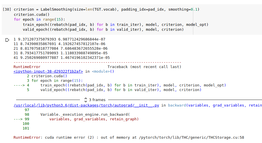
Today we had a look at the Encoder-Decoder architecture and setup and bugfixed the annotated ipynb on Google Colab. You can find it in the overall implementation at the bottom. Unfortunately this implementation doesn’t work as of today, as we soon run out of memory on the free Colab tier:

Therefore, I’ll continue tomorrow on some stronger machine.

Overall implementation

You can download all of this including Sasha Rushes and my notes from here: https://colab.research.google.com/drive/1tm0_Usqkavr0h1Jk0f-ukcykI78xmcfW.

Sources

• https://github.com/harvardnlp/annotated-transformer
• https://jalammar.github.io/illustrated-transformer